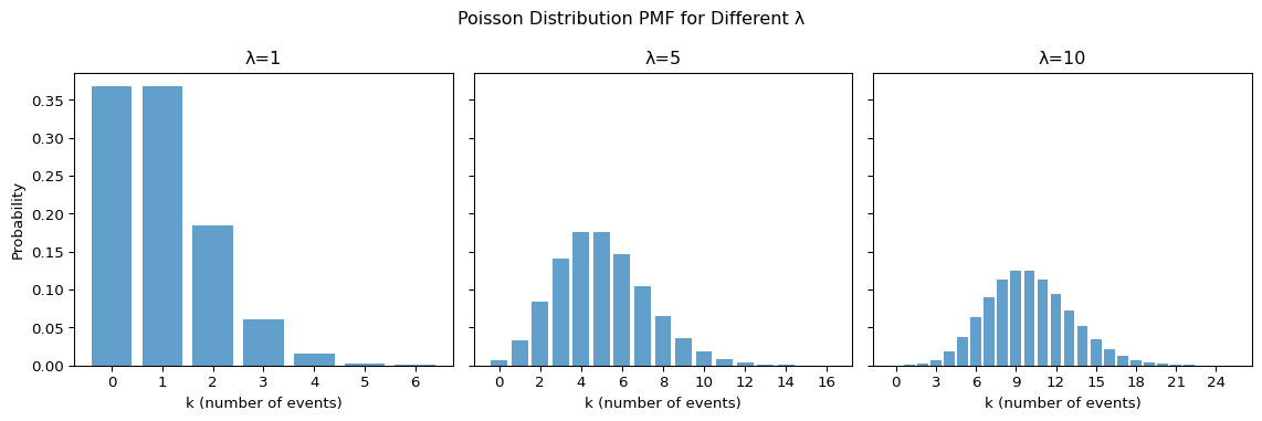
Measuring in Intervals

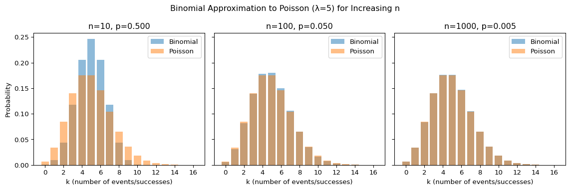
Poisson and Related Distributions

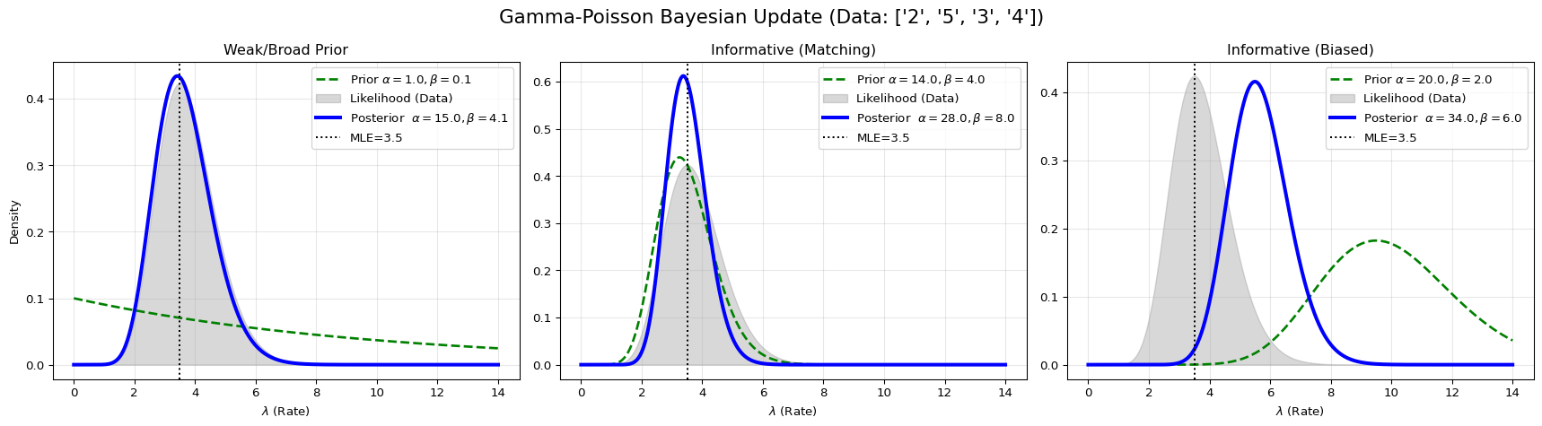
Yu Cheng Hsu

Intended Learning Outcomes

• Characterize Poisson, Exponential, and Gamma distribution
• Apply Bayesian priors for Poisson, Exponential, and Gamma distribution

Observation in a Fixed Time Interval

Poisson Distribution

The Poisson distribution expresses the probability of a given number of events occurring in a fixed interval of time if these events occur with a known constant mean rate and independently of the time since the last event.

• Support \(x \in \mathbb{N}\)
• Parameter \(\lambda\), arrival rate.
• pmf

\[ P( X = x) = \frac{\lambda^x}{x!}\exp(-\lambda) \]

Properties

• Mean \(\lambda\)
• Variance \(\lambda\)

Analogy

• Number of cars waiting for traffic lights
• Biological signals (neuron spike, ECG spike)
• Prevalence rate of a disease

Illustration

Binomial Distribution Approximates Poisson Distribution

When \(n \rightarrow \infty\) and \(p \rightarrow 0\), the Binomial distribution approximates the Poisson distribution. In this case, \(\lambda = np\). (Proofs is in the tutorial question)

Implication

• \(n \rightarrow \infty\), and \(p \rightarrow 0\) implies rare event for Poisson distribution
• Rule of thumb: \(n \geq 100\) and \(np \leq 10\)

Illustration

Negative Binomial Distribution Approximates Poisson Distribution

When \(r \rightarrow \infty\) and \(p \rightarrow 0\), the Negative Binomial distribution approximates the Poisson distribution. (Proofs is in the tutorial question)

Implication

• \(r \rightarrow \infty\) implies rare event to call a stop
• Rule of thembs: \(r \geq 10\) and \(rp \leq 10\)

In practice, the negative binomial distribution is more popular than Poisson distribution

Illustration

Observation in a Fixed Count

Exponential Distribution

A random variable describing the time (or distance) between two Poisson arrivals. If \(X\) is an event count that follows \(X \sim \text{Poisson}\left( \mu \right)\), then the time \(T\) between events follows \(T \sim \text{Exponential}( \frac{1}{\mu})\).

Properties

• Support \(x > 0\)
• Parameter \(\lambda\), arrival rate.
• pdf

\[ f_X( x ) = \lambda e^{-\lambda x} \]

• Mean \(\text{E}(X) = \frac{1}{\lambda}\)
• Variance \(\text{V}(X) = \frac{1}{\lambda^2}\)

Example

• Waiting time for the next bus if arrivals are Poisson
• Waiting time for developing cancer after exposure

Example in population genetics

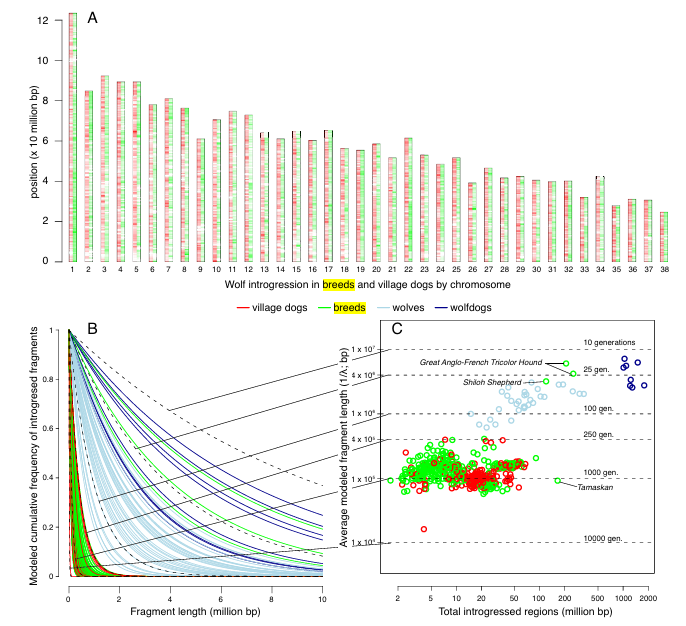
Our dog is dog or wolf Lin et al. (2025)

• Traaditional theory think dog (Canis lupus familiaris) and wolf (Canis lupus) are two differnet species (i.e Monophyly)

• Recent study shows that from a wild range of village dogs gene we can almost reconstruct a wolf’s gene
• Wolf’s gene are just fragmented in dogs gene depends on species
• Based on the fragmented size we can estimate how long does it happened (i.e. small fragmented means happened in long time ago)

dog-wolf introgression

Conjugate Prior

Gamma Distribution

Let \(x_1,\dots x_n\) be i.i.d random variables from an exponential distribution \(\lambda\), then \(\sum_{i=1}^nx_n \sim \text{Gamma}(n, n\lambda)\). Gamma distribution can be used to describe time elapsing until the accumulation of a specific number of unpredictable events.

Properties

• Support \(x \in \mathbb{R}\)
• Parameters \(\alpha, \lambda\)
• pdf

\[ f_X\left( x \right) = \frac{\lambda^\alpha}{\Gamma(\alpha)} x^{\alpha - 1} e^{-\lambda x} , \]

1. It is clear that \(\text{Gamma}(1,\lambda)\sim \text{EXP}(\lambda)\)
2. Measurement on time and count.¹
   • \(X\sim\text{Gamma}(\alpha,\lambda)\), and \(Y\sim\text{Pois}(x\lambda)\)
   • \(P(X>x) =P(Y<\alpha)\)

1. An example is that we describe the time to see a bus, so the probability of waiting for more than \(x\) minutes is equivalent to the probability of seeing no bus in \(x\) minutes.

Poisson Distribution with Gamma Distribution Prior

The Gamma distribution is a conjugate prior to the Poisson distribution. Let’s say we have \(n\) observations \(x_1, \dots x_n\) from an unknown Poisson distribution, and we assume the prior probability of \(\lambda \sim \text{Gamma}(\alpha,\beta)\). The posterior estimation of parameter \(\lambda\)

\[ \begin{align} p(\lambda\mid x_1\dots x_i) \propto & \quad p( x_1\dots x_i \mid\lambda)\text{Gamma}(\alpha,\beta) \\ \propto & \quad e^{-n\lambda}\lambda^{\sum x_i}\lambda^{\alpha-1}e^{-\beta\lambda} \\ \propto & \quad \lambda^{\alpha+\sum x_i-1}e^{-(n+\beta)\lambda} \end{align} \]

The posterior distribution: \(\lambda \sim \text{Gamma}(\alpha+\sum x_i,\beta+n)\)

Analogy

Adding pseudo Poisson observations with total \(\alpha\) occurrences in the \(\beta\) time intervals.

Illustration

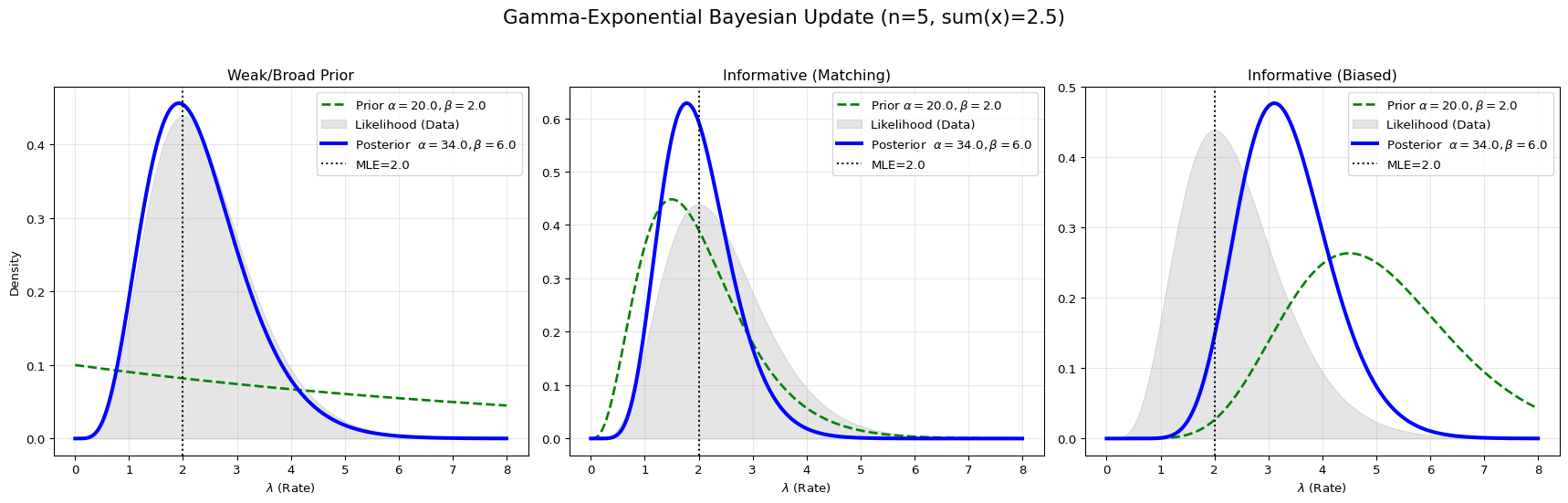
Posterior predictive distribution

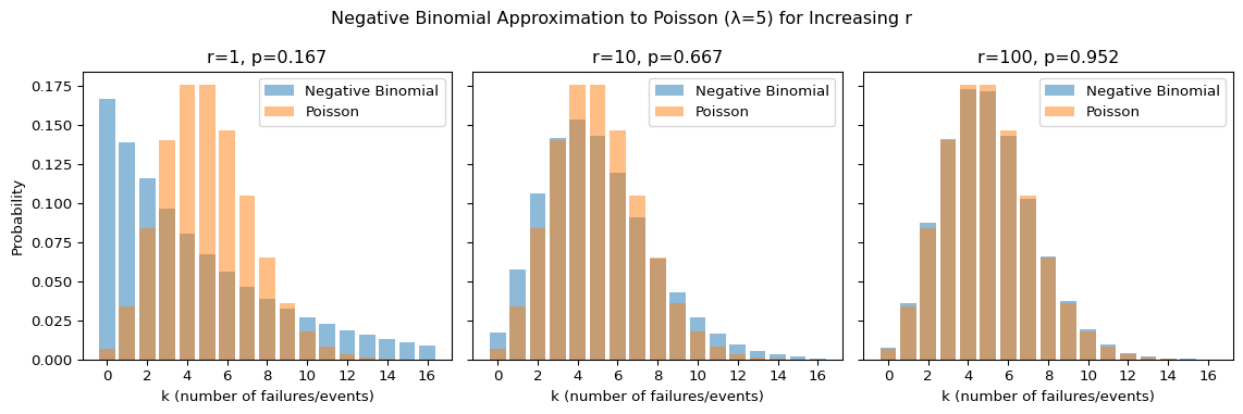
The posterior predicitive distribution of \(p(\tilde{x}|\text{data})\) follows Negative binomial distribution

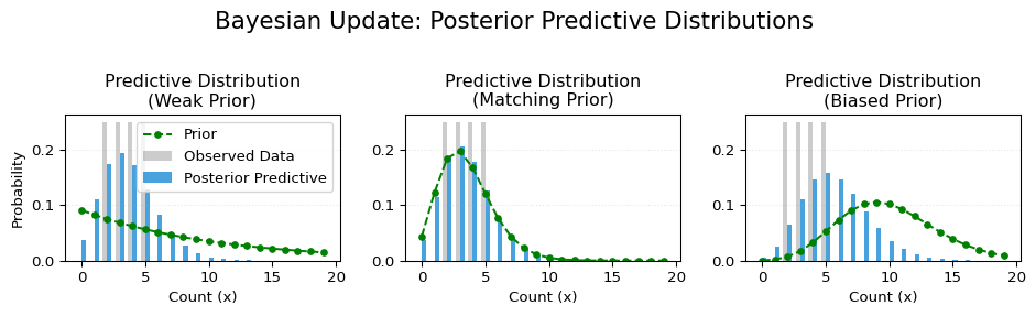
The prove is trivial, but the takeaway is

• Negative binomial distribution can be seen as a Poisson with prior distribution
• Relaxation on variance
• Relatxation comes form the uncertainty of \(\lambda\)
• Zero-inflated data

Exponential Distribution with Gamma Distribution Prior

Let’s say we have \(n\) observations \(x_1, \dots x_n\) from an unknown Exponential distribution, and we assume the prior probability of \(\lambda \sim \text{Gamma}(\alpha,\beta)\). The posterior estimation of parameter \(\lambda\)

\[ \begin{align} p(\lambda\mid x_1\dots x_i) \propto & \quad p( x_1\dots x_i \mid\lambda)\text{Gamma}(\alpha,\beta) \\ \propto & \quad \lambda^n e^{-\lambda \sum x_i }\lambda^{\alpha-1}e^{-\lambda\beta}\\ = & \quad \lambda^{n+\alpha-1}e^{-(\sum x_i+\beta)\lambda} \end{align} \]

Posterior distribution: \(\text{Gamma}(n+\alpha,\sum x_i +\beta)\)

Analogy

Adding pseudo observations with total \(\alpha\) observations over total time \(\beta\)

Illustration

Quick Review

Quick Review

Distribution	Parameter	Conjugate Prior	Posterior Hyperparameters	Posterior Predictive
Bernoulli	\(p\)	\(\small\text{Beta}(\alpha,\beta)\)	\(\small\begin{aligned}\alpha' = \alpha+\sum x_i, \\ \beta'=\beta+n-\sum x_i\end{aligned}\)	\(\small\text{Bern}(\frac{\alpha'}{\alpha'+\beta'})\)
Binomial	\(p\)	\(\small\text{Beta}(\alpha,\beta)\)	\(\small\begin{aligned}\alpha' = \alpha+\sum x_i, \\ \beta'=\beta+\sum n-\sum x_i\end{aligned}\)	\(\small\text{Beta-binomial}(\alpha',\beta')\)
Negative Binomial	\(p\)	\(\small\text{Beta}(\alpha,\beta)\)	\(\small\begin{aligned}\alpha' = \alpha+rn, \\ \beta'=\beta+\sum x_i\end{aligned}\)
Geometric	\(p\)	\(\small\text{Beta}(\alpha,\beta)\)	\(\small\begin{aligned}\alpha' = \alpha+n, \\ \beta'=\beta+\sum x_i\end{aligned}\)

Quick Review

Distribution	Parameter	Conjugate Prior	Posterior Hyperparameters	Posterior Predictive
Poisson	\(\lambda\)	\(\small\text{Gamma}(\alpha,\beta)\)	\(\small\begin{aligned}\alpha' = \alpha+\sum x_i, \\ \beta'=\beta+n\end{aligned}\)	\(\small\text{NB}(\alpha',\frac{\beta'}{1+\beta'})\)
Exponential	\(\lambda\)	\(\small\text{Gamma}(\alpha,\beta)\)	\(\small\begin{aligned}\alpha' = \alpha+n, \\ \beta'=\beta+\sum x_i\end{aligned}\)	\(\small\frac{\beta'}{\alpha'}(1+\frac{x}{\alpha'})^{-\beta'-1}\)

Bibilography notes

Lin, Audrey T, Regina A Fairbanks, Jose Barba-Montoya, Hsiao-Lei Liu, and Logan Kistler. 2025. “A Legacy of Genetic Entanglement with Wolves Shapes Modern Dogs.” Proceedings of the National Academy of Sciences 122 (48): e2421768122.